Understanding the Value of Uniswap v3 Liquidity Positions
See part 1 and part 2 of this series to learn about how Uniswap v3 LP tokens effectively behave like short puts and short calls.
Uniswap has revamped the way liquidity positions are created and managed in version 3 of their protocol. Compared with Uniswap v2, the process to establish a new position is fairly complex. If you’re like me, you may simply click the + New Position button and adjust the range and parameters until you get something that looks good enough. What’s the best way to choose the parameters of a LP position?

In this article, we will describe what happens under the hood when a LP position is created. We will also derive a set of simple set of relationships that may help in choosing the optimal range of Uniswap v3 LP positions across many underlyings.
What is the value of a Uniswap v3 LP token?
The Uniswap v3 whitepaper describes how much of each asset has to be added when establishing a new position. The number of token0 and token1 in a new LP position will depend on the range determined by the lower tick tL, the upper tick tH and the price at entry P0.
I am reprinting equations (6.29) and (6.30) from the whitepaper in a slightly different notation to show how tL and tH are related to P0:

Here, the value of ∆E is determined by the initial amount token0 (denoted by x0) and token1 (denoted by y0) that is locked into the position when it is established:

Once the position is established, we can compute its Net Liquidity Value by adding the amount of token1 to the amount of token0 times the price P:

If the price is above the upper tick tH, the Net Liq value of the LP token will converge to the geometric mean √(tL*tH). When the price is below the lower tick tL, the value of the LP token will simply be P times the size of the position.
When the value is between ticks tL and tH, the expression is a bit more complicated and depends on a function of the square root of the price P. Graphically, here’s what the Net Liq value V(P) looks like:

Changing the range (tL, tH) changes the “sharpness” of the payoff curve V(P). The curve V(P) will converge to the dashed line in the figure above when (tL,tH) is a single tick wide. Again, a 1–tick wide LP position is exactly the return function of a covered call at expiration, without considering the collected fees.
Computing Delta, the rate of change in Net Liq Value
How will the value of a LP position be affected by the price of the underlyings? Specifically, we’d like to know how much would the Net Liq change if the value of token0 changes by $1. This quantity is called “delta” and represents the price sensitivity of an option.
We can obtain δ(P) by taking the partial derivative of the Net Liq value function V(P) with respect to the price P to get the following expression:

It is much easier to understand this expression if we look at it graphically and normalize by the value of the position ∆E. Since the derivative of a function is its instantaneous slope, the value of delta is simply the slope of a line that is tangential to the price curve V(P):

What this figure represents is how much the value of a LP token tracks the price of the underlying. Delta goes from 1 to 0 as the price increases, meaning that the value will match the price of the underlying with 100% correlation at low prices and 0% above the upper tick.
More concretely, let’s consider a LP position deployed between (2000, 3000) that accrues 30% APR from the collected fees. You can think of delta as the slope of the blue line divided by the slope of the red line. Since the value of δ(P) is always less than or equal to 1, the return of a LP position will also be less than or equal to a holding strategy.

Notice the rather large discrepancy between the ETH price and the LP position when the price is above 3000. The area between the red and blue curve is referred to as the impermanent loss (IL). Some will see IL as “missing a great opportunity for profits” and many are extremely worried about it.
Impermanent loss doesn’t worry me at all because I understand that this “missed opportunity” is a feature of covered call positions. As I described in a recent series of tweets, while LP positions do suffer from impermanent loss, LP positions actually decreases the volatility of portfolio returns:
Understanding the impact of Net Delta on returns
Why do we care about delta? Understanding a portfolio’s delta can help manage risks and reduce returns volatility. Hedge funds typically need to compute the delta of their financial instruments to create a portfolio containing many assets structured in way that is delta neutral — ie. whose total value will remain constant despite market swings.
The short strangle and short straddles I created in my previous post are two examples of strategies that limit exposure to price fluctuations (delta=0). My hope is that these positions will maintain their value by limiting “impermanent loss” and turn in a profit by accumulating fees. (update: they’re still profitable with 7 days to go until “expiration”!)
Or, it may be beneficial to have a negative delta so that the value of a portfolio increases when the price of the underlying decreases. This is true especially when considering a LP position that is established between ETH and another token. Many DeFi tokens have underperformed ETH in the past 6 months even though their value increased when denominated in stablecoin. An investor may wish to hedge against underperforming assets by creating a short call position.
Therefore, to understand how the value of a portfolio will fare against both upward and downward moves across many assets, we need to know what is the Net Delta of a portfolio. We’ll illustrate how to do this with a hypothetical portfolio consisting of 3 LP positions: ETH/Dai, ETH/UNI, and ETH/WBTC. The parameters of each LP position are summarized below.

Here, we introduce beta (β), a quantity that tracks the correlation to a reference asset. Using beta, we can calculate the portfolio’s Net Delta according to the delta of each asset weighted by beta (here I express delta in terms of ETH to simplify the calculation):

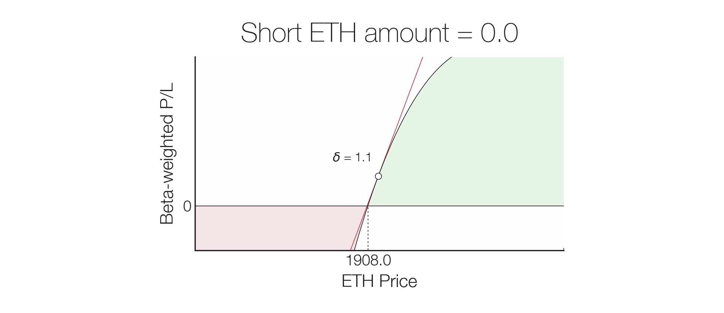
Using the information from the table above, we get that the net delta of our portfolio is 1.126. This means that the value of our portfolio — which contains a rather complex mix of ETH, Uni, and WBTC LP positions — will change by $1.126 for every $1 change in the value of ETH.
One way to look at it is that while combined Net Liq value of the portfolio is 2.69 ETH, the relative change in expected returns following the change in the price of ETH will only be equivalent to a holding with 1.126 ETH, about 60% smaller. While this means smaller returns, it also means lower portfolio volatility.
Another way to use the net delta of a portfolio would be to use it to determine the size of a short position that would neutralize delta and bring it to zero to hedge against small changes in ETH price and help maintain portfolio value. Here’s what the P/L of the position above would look like for different amounts of shorted ETH.

Future work
In this post, we derived an expression for the total value of a Uniswap v3 LP position. We found that the price sensitivity of a Uniswap v3 LP option can help understand future returns, and we described a procedure for calculating the delta of a portfolio composed of many Uniswap v3 LP pairs.
The discussion above may have been familiar for those that know about the Black-Scholes model and “the Greeks” for options derivatives. Beyond delta, other relevant quantities to consider are gamma = dδ/dS, theta=dV/dt, and vega=dV/dσ.
Each has their role to play in determining the returns of a portfolio, and we will expand the use of these parameters in the next post to derive the expected return on investment for Uniswap v3 options using “Black-Scholes”-like pricing models based on Geometric Brownian Motion.
Stay tuned!
If you’re interested in these ideas and would like to contribute to the development of a UI interface for trading Uni v3 options, please DM me on twitter @guil_lambert or send an email to guil.lambert @ protonmail.com
