A Guide for Choosing Optimal Uniswap V3 LP Positions, Part 1

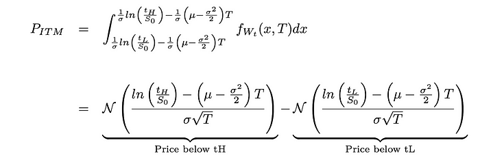
TL;DR: the probability that a LP position centered between an upper tick tH and a lower tick tL will end up within that range (ie. be In-The-Money) after a time T is:

For more details, read my post below.

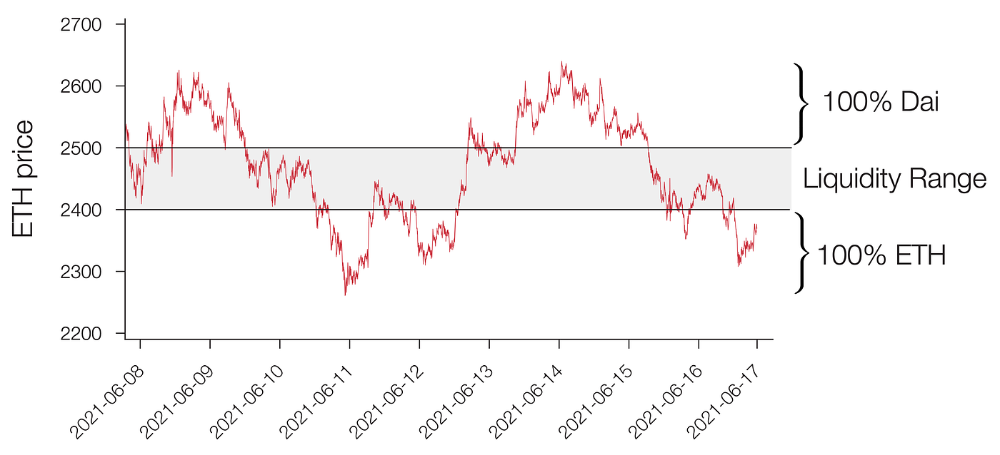
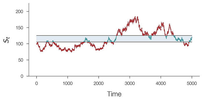
Choosing a liquidity range for Uniswap v3 LP tokens can be difficult. In the example above, the deployed liquidity will be converted to 100% Dai above 2500 and to 100% ETH below 2400. For large price swings, a liquidity position may suffer impermanent loss and positions outside of their defined ranges won’t be able to benefit from capital appreciation.

Since deploying liquidity in Uniswap v3 is rather complicated, users can be tempted to pool their liquidity with other users and trust the active management of liquidity positions (see this great review post by @vividot).

However, for users that still want to manage their own position, several questions exists as to how to best deploy liquidity in Uniswap v3:

1. What should the center price be?
2. What should be the value of the upper and lower ticks?
3. What is the likelihood that the price of a given asset will remain within a specified price range after a certain time?
4. How long to keep a position on?
5. What’s a realistic profit target?

In this post, I will attempt to answer these questions in a quantitative manner using mathematical models of asset pricing. It turns out the solution to these questions is rooted in the behavior of Geometric Brownian Motion. But feel free to directly use the result from the TL;DR above if you don’t want to follow along :)

Expected move of a crypto asset price

A modern view of asset valuation is that the price of any instrument (stock, bond, options, derivatives) is stochastic and evolves randomly over time.

Geometric Brownian Motion. 500 simulations of the price of an asset using the Geometric Brownian Process. We should expect the majority of the traces to remain within the expected move (dashed lines)

Specifically, the pricing of an asset has a drift μ and a volatility σ will be described by a stochastic partial differential equation (PDE) given by:

You can think of the drift μ as the expected long-term return. For example, the S&P500 has averaged an annual return of approximately 10% over the past 50 years. So the drift term in that case would be 0.1/year.

The volatility σ, on the other hand, describes how much the price at any given instant is prone to stochastic variations around that expected return. The historical volatility of the S&P500 oscillates between 10% and 30% depending on the frothiness of the market (see VIX index).

Each asset behaves differently, and each one has their own drift and volatility terms. Crypto assets can be much more volatile than regular stocks and some cryptocurrencies trading pairs may even have a negative drift term. But regardless of the drift and volatility values, the stochastic PDE describing Geometric Brownian Motion can be solved exactly and has solution:

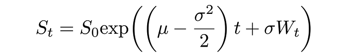
Here, W_t describes a Brownian motion (it is also called a Wiener process). A Wiener process is a series of numbers sampled from a normal distribution with mean equal to 0 and variance equal to 1.

If we choose the volatility σ of a crypto asset like Ether to be between 100% to 150% per year (using data from Genesis Volatility or the Opyn options analytics page) and a drift term μ of less than 1% per year, then most of the numbers in the expression above will be somewhat small compared to 1 for short time intervals (for instance μ-σ²/2 = 0.008 in that case).

This means we can ignore the term multiplying t and Taylor expand the exponential function to get:

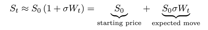
Note that the average displacement of a Wiener process W_t after a time T is simply ±√T. Therefore, the expected move of a crypto asset after a time T is:

Hence, if one were to create a LP position starting at a price S0, there would be a 68% chance (ie. 1 standard deviation) that the asset will move less than S0*σ*√T away from the starting price, either up or down.

ETH Expected Move. Historical ETH price, with the expected move after July 25th (result from 100 simulations). The expected move starting at a price S0 should be ±S0*σ*√T with 68% probability.

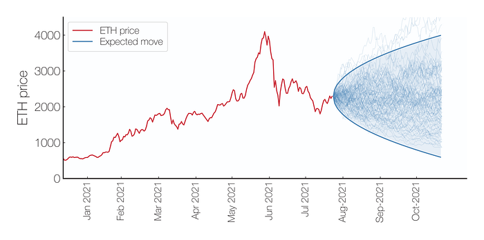
Extending this further, there would be a 95% and 99.7% chance that it would stay within 2x and 3x the expected move, respectively.

Takeaway 1: One must take the expected move of a crypto asset AND a time horizon when choosing the range of a LP position. The expected 1-standard deviation move of an asset after a time T is (S0σ√T), where S0 is the starting price.

Probability of ending up inside a defined range

Having solved the Geometric Brownian Motion stochastic PDE, we next can ask the probability that the price of an asset will end up within an upper and lower tick of a Uniswap LP position after a time T.

Geometric Brownian Motion and Boundary Crossing. What is the probability that a Geometric Brownian Motion will stay within a range defined by a lower and upper tick?

To answer this question, we must invert Eqn. 1 and solve for W_t to get

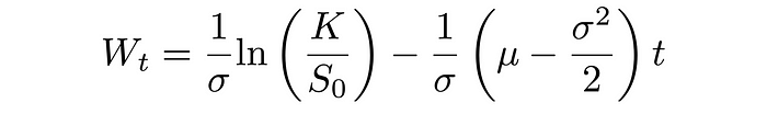
So, asking when the price of an asset will cross a price K when the price starts at S0 is equivalent to asking the probability that a Brownian Motion will cross a moving boundary of the form a+b*t, where a = 1/σ ln(K/S_0) and b = -1/σ(μ-σ²/2).

Wiener Process and Moving Boundary Crossing. Brownian motion is centered around zero and has a variance equal to 1. The boundary is now moving with the price.

Since a Brownian Motion/Wiener process is much simpler to analyze than a Geometric Brownian Motion, we can solve this probability exactly using the probability density function of a Wiener process

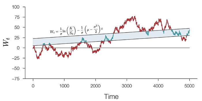
Using this to find the probability that the price is within the wedge defined by the a lower tick tL and upper tick tH at time T (ie. the position ends “in-the-money”), we get

where T = (number of days)/365 and N(x) is the cumulative normal distribution, given by

This expression is a bit complex, but we can first assume that the upper and lower ticks are centered around the current price, and the upper/lower ticks are defined by a range factor r such that:

Then, the expression for P(ITM) can be visualized graphically and it will correspond to the area under the normal distribution curve with mean 0 and standard deviation 1:

Probability of ending In-The-Money. Choosing a Uniswap LP position defined by range 20% above and 20% below a strike results in a probability of ending In-The-Money that depends on the duration T. In this figure, μ= 1%/year and σ= 100%/year.

For a short duration T, the term d0 approaches zero and the upper and lower boundaries converge to +/-ln(r)/σ√T. In that case, the expression for the probability that the position ends In-The-Money reduces to

Since the two term are very similar, we can combine them and transform the cumulative normal distribution into the error function to get:

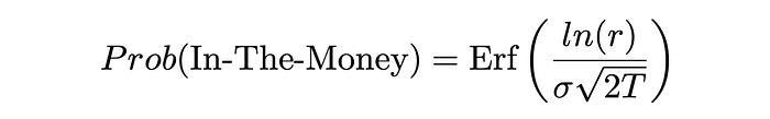
Thankfully, this expression is much simpler and the erf function can actually be computed in Excel, Google Sheets, or by googling it directly.

The expression for P(ITM) should help LP define a range for their position. Ideally, one must choose a range defined by a range factor that maximizes the probability that the price will remain within the LP range and generate fees.

As an example, I’ve created the table below to show the probability of ending in the money for different time windows and range factors:

Probability of ending in-the-money for various duration in days and range factors r. The range factors of 1.001, 1.006 and 1.02 correspond to a 1-tick wide liquidity for the 0.05%, 0.3%, and 1% fee tiers.

Hence, a new LP position must be established with a specific time horizon in mind. For example, a very narrowly defined LP position may “evade” impermanent loss if it is removed after less than a day. On the other hand, holding a very wide LP position for a short amount of time may dilute the liquidity too much and collect a very small amount of fees.

Takeaway 2: The relationship between the upper/lower ticks and the time horizon of a LP position can be visualized graphically, and it converges to P(ITM) = Erf(ln(r)/σ√(2T)).

Towards an optimal Uni v3 LP position?

In this post, we derived an expression for the probability that an asset will end within a specific range after a time T. We found that the expected move of a crypto asset can be predicted using a relatively simple equation, and we derived an expression for the In-The-Money probability that will help liquidity providers choose a range for their LP positions.

While writing this article, I realized that several questions still remain unanswered. While we calculated the probability that a position will end ITM after a time T, what about the fraction of time spent ITM after a time T? In other words, what is the expected amount of fees to be collected for a given range factor?

Uni v3 LP positions never expire, so a position that is Out-The-Money can become ITM and back again with price movements. The LP position will collect 0.3% in fee every time it does so, which can potentially generate large returns under highly volatile conditions. What is the expected return from these swap events?

Analyzing the returns of LP positions as covered calls also adds another layer of complexity to expected returns. Can a market exist where LP tokens are exchanged and priced at a premium due to the potential of future returns?

All these phenomena will impact the pricing and may increase the potential returns of an LP position. I will stop my analysis for now and will cover the rest of LP position returns in part 2 of this post.

Stay tuned!

If you’re interested in these ideas and would like to contribute to the development of a UI interface for trading Uni v3 options, please DM me on twitter @guil_lambert or send an email to guil.lambert @ protonmail.com